Quantifying perineural Invasion in Duplex IHC

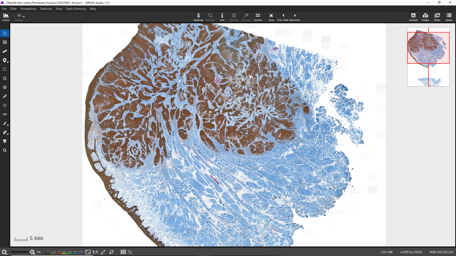
This MIKAIA^® App Note shows how to quantify tumor in proximity to nerve fibers (perineural invasion) in a IHC duplex-stained tissue section, where nerves appear red (antigen: S100) and tumor brown (antigen: cytokeratin):

This App note is created with MIKAIA^® studio 1.5.1.

The overall analysis workflow can be outlined in 3 simple steps:

1. mask nerve fibers using Mask by Color App (color-picker mode: mask red areas)
2. create nerve proximity ROIs by creating concentric margins (0-100 µm and 100-200 µm) around all nerve fiber annotations using the “Add Margins” feature
3. mask tumor using Mask by Color App (stain deconvolution mode: mask brown areas) and separate into ROIs (nerve margin 1, nerve margin 2, rest)

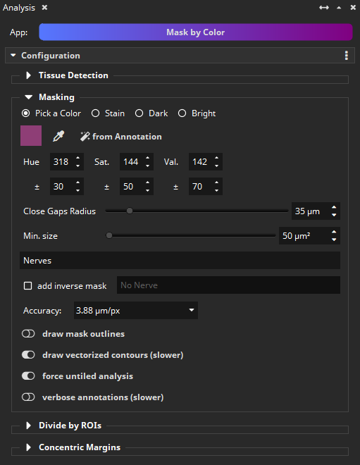
Step 1) mask nerves

Nerves appear red or purple in the scan. These areas can be masked using the Mask by Color App. Select the “Pick a Color” mode and then use the pipette to pick the nerve color (purple). Provide a bit of tolerance (+- 30/50/70 in H/S/V color space, which translates to hue, saturation and brightness). Optionally, specify a minimum nerve fiber area in µm² to prevent that too many very small (false?) objects are detected. Enter “Nerves” as a class name. We select the analysis resolution of 3,88 µm/px. Important: enable the vectorization of contours, so that nerves subsequently become individual polygons, which is a requirement for the “add margins” feature that will be used in the next step.

As a result of this analysis, a single class “Nerves” and detected objects are masked here in yellow. The “Results” panel displays a diagram of the overall footprint of all nerves (in mm²) in contrast to the analyze area.

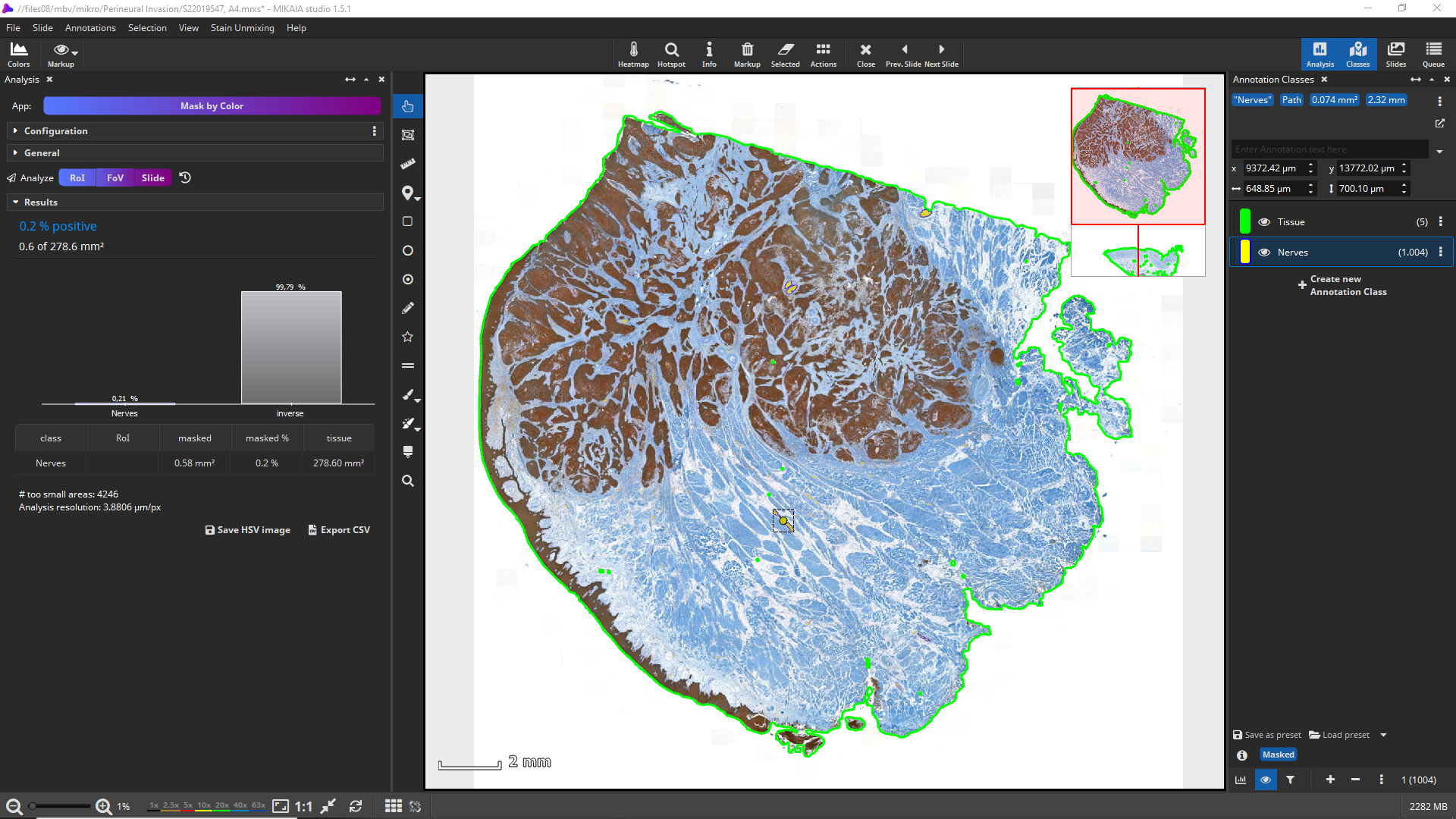
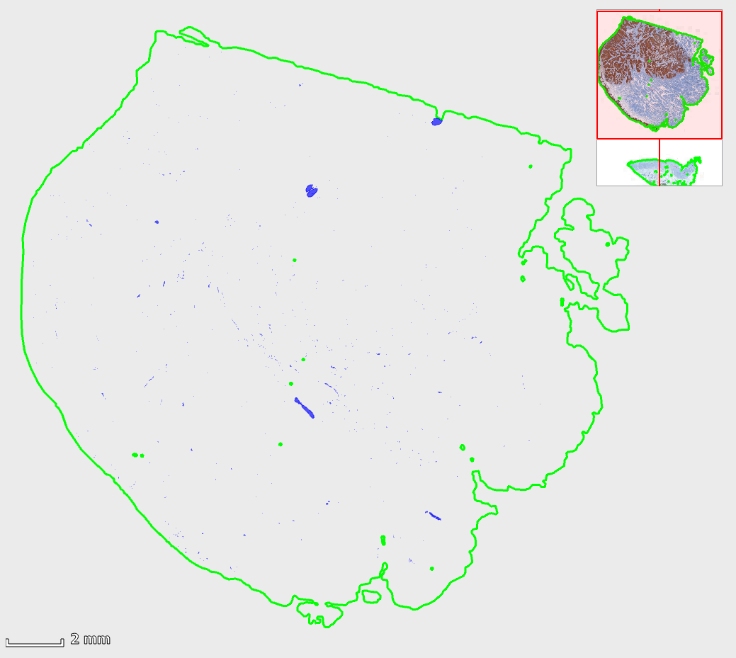
The detected nerve fibers (below in blue) are better visible by temporarily hiding the image (toolbar | Markup | toggle “hide image”):

Step 2) Create nerve proximity masks

Now that nerves have been masked, the next step is to create ROIs of the areas close to a nerve fiber. This will enable us to then measure the presence of tumor in these ROIs in the final step.

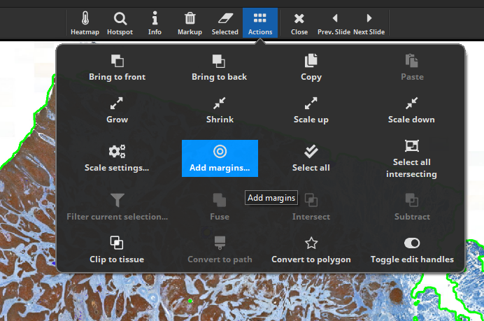
To add margins to all nerve fibers, select at least one fiber and then click “Add margins…”.

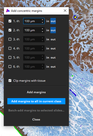
Here, we choose to add 2 concentric outwards margins of a diameter of 100 µm each (this is an arbitrary choice). Click “Add margins to all in current class”.

After a few seconds, two margins are added to all nerve fibers (blue: nerves, dark green: margin 0-100µm, light green: margin 100-200µm). Overlapping margins from adjacent nerve fibers are automatically fused, All margins are clipped to the detected tissue (foreground).

Here is a closeup and the “nerve”-masks are hidden to illustrate how now the proximity of nerves is masked.

Step 3) Mask Tumor

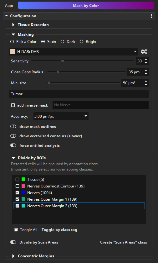
The final step is to mask the tumor and intersect it with the nerve proximity ROIs. Again, the Mask by Color App is used, but now in the “Stain” mode. Select the “H-DAB: DAB” scheme, which performs a H-DAB stain deconvolution and then masks the DAB stain component. Important: enter a different class name or else the previously created mask will be replaced. We use “Tumor” here. Vectorization of the resulting mask can be disabled now to save computation time.

Important: In the “Divide by ROIs” section, select that the tumor mask shall be intersected with the proximity margins. Since the resulting mask will also cover the nerves (purple is closer to DAB/brown than to hematoxylin/blue), select the “Nerves” class as a third ROI, so that its contribution can later be ignored.

The analysis again takes a few seconds and then the DAB stained areas are masked. This time, not a single class “Tumor” is created, but instead multiple tumor classes: tumor in margin 1 (red), tumor in margin 2 (orange), tumor in nerves (hidden) and tumor in rest (yellow). The sizes in mm² of the individual subareas of the tumor mask are shown in the diagram.

This close-up better shows how the tumor area in proximity to nerve fibers is now accurately quantified.

This analysis can also be carried on an entire dataset comprising many slides. After good parameters have been selected by experimenting with one or a few slides, each step above can be run as a batch-analysis on many slides. The quantitative results, in particular the areas in µm² of the individual masks are all exported to a CSV file that can be opened in Microsoft Excel or imported with R, Python or Matlab to generate diagrams.

Please also check out other App Notes in the MIKAIA^® University.

Image copyright: Fraunhofer IIS