IHC Profiler in MIKAIA – Assessing New IHC Assay Using Multi-organ TMA

When designing a new  immunohistochemistry (IHC) assay, a quantitative assessment of how it “responds” in different tissues of various organs is insightful and helps optimizing the assay in an objective way. In the following use case, the IHC Profiler in MIKAIA is utilized for the quantitative evaluation of tissue microarray (TMA) cores from various tissue samples.

Objective

In this MIKAIA University application note, the researchers’ objective was to quantify and grade separately

• the stain intensity per TMA core
• the positive area per TMA core.

Why are intensity and area assessed independently? This is simply due to the fact that it is hardly possible to source TMA cores from the various tissues in a standardized way, with always the exact same ratio of tissue expected to be positive or negative. It is in the nature of a specific IHC assay that it stains only desired antigens and does not yield a response in the remaining tissues. Therefore, a larger positive area in a TMA core is not per se a good or bad result.

The stain intensity, on the other hand, states how strongly the chromogen, e.g., DAB in this use case, is visible. Here, a stronger intensity is typically desired.

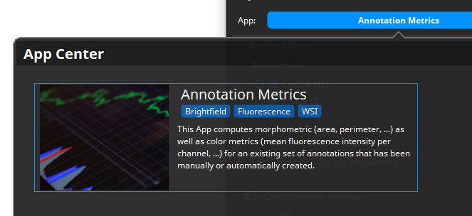
The MIKAIA Annotation Metrics App can be used in this scenario. The app will iterate over existing annotation objects in a given annotation class (or multiple classes) and calculate a set of metrics for each annotation. The annotations to be analyzed can either be drawn manually or one of the other apps can be used.

Detecting TMA cores

Here, the Tissue Detection App was used to automatically detect all TMA cores first. The app is used to batch-analyze all whole-slide-images (WSIs) in the dataset with the “save in place” option enabled. Subsequently, the detection results should be checked and annotations can be corrected wherever necessary. The magic brush and magic eraser tools, which smoothly align the brush circle to the image contents, are very handy in this step. MIKAIA stores annotations decentrally in a proprietary *.ano file next to the original WSI file. This has the advantage that scans can be moved around to other folders after they have been analyzed. As long as the *.ano file stays next to it, it will be auto-detected by MIKAIA when the slide is opened. Additionally, *.ano annotation files can be easily shared via email. It is good practice and recommended to copy the *.ano files after any analysis step that takes longer or involves manual work, and place them in a separate folder, just to be safe. This way one can later always revert to this stage, if necessary.

IHC Profiler in the Annotation Metrics App

Now that all annotation are available, the Annotation Metrics App can be used to analyze them.

In a minimal setting, it will only calculate morphometric attributes such as the area in mm², the perimeter, the roundness, etc. and export them into a CSV file. Here, however, we are interested in profiling the colors, and so we activate the Calculate the color metrics option. When a brightfield scan is loaded, the app will unmix the stains and then analyze one single stain, i.e., DAB in this example. The app “looks” at the unmixed image in the so called optical-density (OD) color space, where pixels are dark when the chromogen is absent and bright when it is present. Additionally, we select incl. histogram. This way, the color histogram is calculated for each annotation. The histogram provides a good basis for deriving both the stain intensity and the positive area. The histogram states for each color intensity (0-255) the number of pixels with this color intensity. The unit written to the CSV file can be pixels, µm² or normalized (i.e., the sum of all values is 1.0).

In fact, the IHC Profiling could then take place within Excel or any other statistics/plotting tool that can read in the exported CSV (e.g., Matlab, Python, R). But it is helpful to get a visualization of the detected grades.

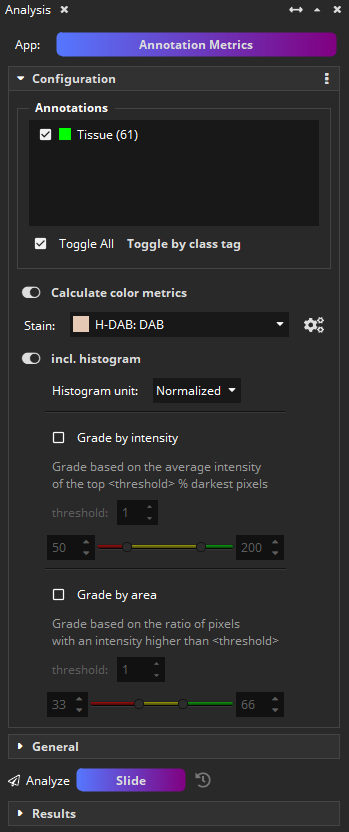
When the Grade by intensity option is selected, the app will generate new annotations and assign them into one of the classes Intensity – low, Intensity – medium, or Intensity – high. The grade is computed by computing the mean value of the darkest N % pixels in the annotation. The N (default: 5 %) as well as the cut-offs for low/medium/high can be configured.

When the Grade by area option is selected, the app will additionally generate another set of new annotations and assign them into one of the classes Pos. Area – low, Pos. Area – medium, or Pos. Area – high. The grade is computed by computing the ratio of pixels that is darker than a threshold T. The T (default: 64) as well as the cut-offs for low/medium/high can be configured.

When enabling both grades, be careful to visualize only one set of grade-classes as the annotations overlap each other. The classes are tagged either with the Intensity tag or the Pos. Area tag. Clicking a tag button (bottom of Annotation Classes sidebar) will automatically toggle the visibility of all classes with this tag.